Frequentist methods make promises about procedures: if you follow the plan, you will wrongly claim an effect in at most α of the studies where none exists. Bayesian methods make statements about this dataset under this model and prior. Here is what happens when researchers peek at their data every 10 participants per group and stop when they like the result. R/simulate_data.R ran 2,000 studies per scenario (a minute or two); we load the summary.
Explainer: false positives, power, peeking
False-positive rate: among studies where the true effect is zero, the share that claim an effect. With p < .05 and one planned analysis, it is 5%.
Power: among studies where the effect is real, the share that detect it (here, reach p < .05).
Peeking (optional stopping): checking results repeatedly as data come in and stopping once they look good. Each extra look is another chance for noise to cross the threshold.
Sequential design: a plan that builds in repeated looks, with thresholds chosen in advance so error rates stay controlled.
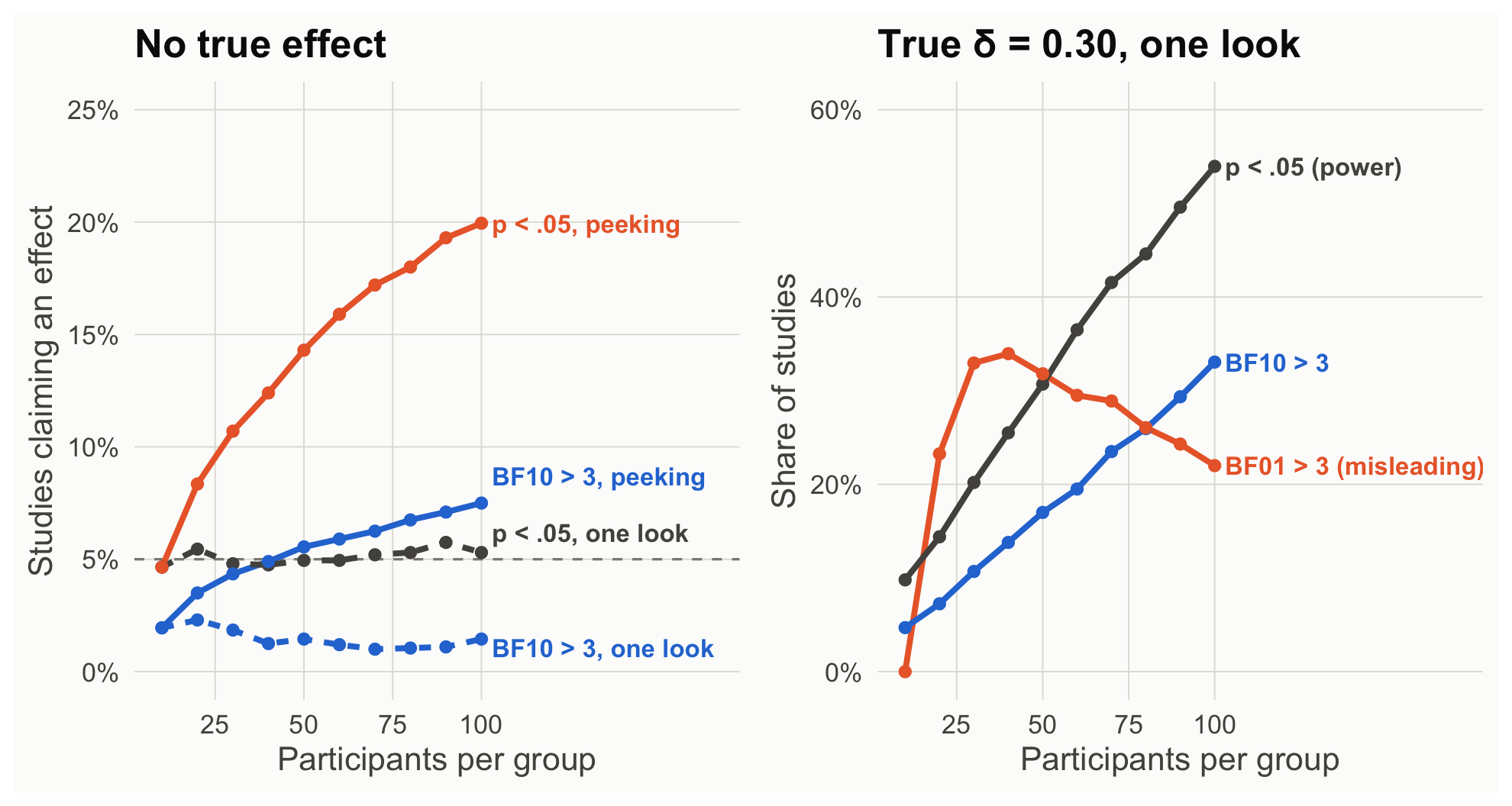
Figure 1: Left: when there is no effect, how often each rule claims one (dashed lines: one look at n per group; solid: peeking every 10 per group). Right: when the true effect is small (δ = 0.30), how often a single look at n per group gives each result.
How to read this figure
Left: studies where there is no true effect. The vertical axis is the share that claimed one; the horizontal axis is how many participants per group had been collected.
Dashed lines: one planned analysis at that sample size. Solid lines: peeking every 10 participants per group and stopping at the first “success.”
Right: studies of a real but small effect (δ = 0.30), each analyzed once at the given sample size. Gray is power; blue is the share with at least moderate evidence for the effect; orange is the share with moderate evidence against it, which is misleading here.
Peeking breaks the p value’s promise. With one look, false positives stay at 5%. Peeking every 10 participants inflates them to about 20%.
Bayes factors are not immune either. BF₁₀ > 3 is a stricter criterion than p < .05 at these sample sizes, so it starts with fewer false alarms (about 1.5% with one look at 100 per group). Peeking still multiplies them, here to about 8%. The Bayes factor still means what it says about the data in hand (Rouder, 2014), but if you act on a threshold, you need to know how often that action misleads, and the guarantees depend on the prior (de Heide & Grünwald, 2021).
Sequential designs have to be planned. Sequential Bayes factor designs set their thresholds and minimum sample size by simulation to keep misleading evidence rare (Schönbrodt et al., 2017). With lax settings (stop at BF 3 or 1/3, first look at 10 per group), 56% of simulated studies of a real δ = 0.30 effect stop with “evidence for no effect.”
Default Bayes factors can mislead toward the null when true effects are small. At 50 per group, 32% of studies of a real δ = 0.30 effect produce “moderate evidence” for no effect, because the default alternative expected bigger effects. This is Scene 2’s lesson again: the prior is part of the hypothesis.
Theory-building takeaway. If your field needs claims that are rarely wrong in the long run, frequentist error control is the tool. If it needs graded evidence among specific theories, Bayes factors are. Either way, plan the analysis before seeing the data.
Source Code
---title: "Scene 6 · What each framework promises"subtitle: "For after class"---```{r}#| label: setup#| include: falsesource("R/helpers.R")suppressPackageStartupMessages({library(BayesFactor)library(patchwork)})knitr::opts_chunk$set(fig.align ="center")```Frequentist methods make promises about **procedures**: if you follow the plan, you will wrongly claim an effect in at most α of the studies where none exists. Bayesian methods make statements about **this dataset under this model and prior**. Here is what happens when researchers peek at their data every 10 participants per group and stop when they like the result. `R/simulate_data.R` ran 2,000 studies per scenario (a minute or two); we load the summary.::: {.callout-note collapse="true" title="Explainer: false positives, power, peeking"}- **False-positive rate:** among studies where the true effect is zero, the share that claim an effect. With *p* < .05 and one planned analysis, it is 5%.- **Power:** among studies where the effect is real, the share that detect it (here, reach *p* < .05).- **Peeking (optional stopping):** checking results repeatedly as data come in and stopping once they look good. Each extra look is another chance for noise to cross the threshold.- **Sequential design:** a plan that builds in repeated looks, with thresholds chosen in advance so error rates stay controlled.:::```{r}#| label: s6-loadpeek <-read.csv("data/sim_peeking_summary.csv")knitr::kable(peek[peek$n_per_group %in%c(20, 50, 100), c("true_delta", "n_per_group", "fixed_p05", "peek_p05","fixed_bf10_gt3", "peek_bf10_gt3", "fixed_bf01_gt3")],col.names =c("True δ", "n / group", "p < .05 (one look)", "p < .05 (peeking)","BF10 > 3 (one look)", "BF10 > 3 (peeking)", "BF01 > 3 (one look)"),row.names =FALSE, digits =3)``````{r}#| label: fig-peek#| code-fold: true#| fig-height: 4.8#| fig-cap: "Left: when there is no effect, how often each rule claims one (dashed lines: one look at n per group; solid: peeking every 10 per group). Right: when the true effect is small (δ = 0.30), how often a single look at n per group gives each result."h0 <- peek[peek$true_delta ==0, ]a <-rbind(data.frame(n = h0$n_per_group, rate = h0$fixed_p05, rule ="p < .05, one look"),data.frame(n = h0$n_per_group, rate = h0$peek_p05, rule ="p < .05, peeking"),data.frame(n = h0$n_per_group, rate = h0$peek_bf10_gt3, rule ="BF10 > 3, peeking"),data.frame(n = h0$n_per_group, rate = h0$fixed_bf10_gt3, rule ="BF10 > 3, one look"))h1 <- peek[peek$true_delta ==0.3, ]b <-rbind(data.frame(n = h1$n_per_group, rate = h1$fixed_p05, rule ="p < .05 (power)"),data.frame(n = h1$n_per_group, rate = h1$fixed_bf10_gt3, rule ="BF10 > 3"),data.frame(n = h1$n_per_group, rate = h1$fixed_bf01_gt3, rule ="BF01 > 3 (misleading)"))cA <-c("p < .05, one look"= pal[["ink2"]], "p < .05, peeking"= pal[["orange"]], "BF10 > 3, peeking"= pal[["blue"]], "BF10 > 3, one look"= pal[["blue"]])cB <-c("p < .05 (power)"= pal[["ink2"]], "BF10 > 3"= pal[["blue"]], "BF01 > 3 (misleading)"= pal[["orange"]])lA <- a[a$n ==100, ]; lB <- b[b$n ==100, ]lA$rate <- lA$rate +ifelse(lA$rule =="BF10 > 3, peeking", 0.012, ifelse(lA$rule =="p < .05, one look", 0.009, ifelse(lA$rule =="BF10 > 3, one look", -0.004, 0)))pa <-ggplot(a, aes(n, rate, color = rule, linetype =grepl("one look", rule))) +geom_hline(yintercept =0.05, linetype ="dashed", color = pal[["gray"]]) +geom_line(linewidth =1.2) +geom_point(size =2) +scale_linetype_manual(values =c(`TRUE`="22", `FALSE`="solid")) +geom_text(data = lA, aes(label = rule), hjust =0, nudge_x =3, size =3.8, fontface ="bold") +scale_x_continuous(breaks =c(25, 50, 75, 100), limits =c(10, 165)) +scale_color_manual(values = cA) +scale_y_continuous(labels = scales::percent, limits =c(0, 0.25)) +labs(x ="Participants per group", y ="Studies claiming an effect", title ="No true effect") +theme_demo(14)pb <-ggplot(b, aes(n, rate, color = rule)) +geom_line(linewidth =1.2) +geom_point(size =2) +geom_text(data = lB, aes(label = rule), hjust =0, nudge_x =3, size =3.8, fontface ="bold") +scale_x_continuous(breaks =c(25, 50, 75, 100), limits =c(10, 170)) +scale_color_manual(values = cB) +scale_y_continuous(labels = scales::percent, limits =c(0, 0.6)) +labs(x ="Participants per group", y ="Share of studies", title ="True δ = 0.30, one look") +theme_demo(14)pa + pb```::: {.callout-note appearance="simple" title="How to read this figure"}1. **Left:** studies where there is no true effect. The vertical axis is the share that claimed one; the horizontal axis is how many participants per group had been collected.2. **Dashed lines:** one planned analysis at that sample size. **Solid lines:** peeking every 10 participants per group and stopping at the first "success."3. **Right:** studies of a real but small effect (δ = 0.30), each analyzed once at the given sample size. Gray is power; blue is the share with at least moderate evidence *for* the effect; orange is the share with moderate evidence *against* it, which is misleading here.:::- **Peeking breaks the *p* value's promise.** With one look, false positives stay at 5%. Peeking every 10 participants inflates them to about `r round(100 * h0$peek_p05[10])`%.- **Bayes factors are not immune either.** BF₁₀ > 3 is a stricter criterion than *p* < .05 at these sample sizes, so it starts with fewer false alarms (about `r round(100 * h0$fixed_bf10_gt3[10], 1)`% with one look at 100 per group). Peeking still multiplies them, here to about `r round(100 * h0$peek_bf10_gt3[10])`%. The Bayes factor still means what it says about the data in hand (Rouder, 2014), but if you *act* on a threshold, you need to know how often that action misleads, and the guarantees depend on the prior (de Heide & Grünwald, 2021).- **Sequential designs have to be planned.** Sequential Bayes factor designs set their thresholds and minimum sample size by simulation to keep misleading evidence rare (Schönbrodt et al., 2017). With lax settings (stop at BF 3 or 1/3, first look at 10 per group), `r round(100 * h1$sbf_end_h0[10])`% of simulated studies of a real δ = 0.30 effect stop with "evidence for no effect."- **Default Bayes factors can mislead toward the null when true effects are small.** At 50 per group, `r round(100 * h1$fixed_bf01_gt3[5])`% of studies of a real δ = 0.30 effect produce "moderate evidence" for no effect, because the default alternative expected bigger effects. This is [Scene 2](scene-2.qmd)'s lesson again: the prior is part of the hypothesis.**Theory-building takeaway.** If your field needs claims that are rarely wrong in the long run, frequentist error control is the tool. If it needs graded evidence among specific theories, Bayes factors are. Either way, plan the analysis before seeing the data.